Before analyzing data, a Data Scientist must extract the data, and make it clean and valuable.
Extract and Read Data With Pandas
Before data can be analyzed, it must be imported/extracted.
In the example below, we show you how to import data using Pandas in Python.
We use the read_csv() function to import a CSV file with the health data:
Example
  import pandas as pd

health_data = pd.read_csv("data.csv", header=0, sep=",")

print(health_data)
Example Explained
- Import the Pandas library
- Name the data frame as
health_data. header=0means that the headers for the variable names are to be found in the first row (note that 0 means the first row in Python)sep=","means that "," is used as the separator between the values. This is because we are using the file type .csv (comma separated values)
Tip: If you have a large CSV file, you can use the head() function to only show the top 5rows:
Example
  import pandas as pd

health_data = pd.read_csv("data.csv", header=0, sep=",")

print(health_data.head())
Data Cleaning
Look at the imported data. As you can see, the data are "dirty" with wrongly or unregistered values:
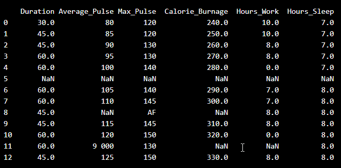
- There are some blank fields
- Average pulse of 9 000 is not possible
- 9 000 will be treated as non-numeric, because of the space separator
- One observation of max pulse is denoted as "AF", which does not make sense
So, we must clean the data in order to perform the analysis.
Remove Blank Rows
We see that the non-numeric values (9 000 and AF) are in the same rows with missing values.
Solution: We can remove the rows with missing observations to fix this problem.
When we load a data set using Pandas, all blank cells are automatically converted into "NaN" values.
So, removing the NaN cells gives us a clean data set that can be analyzed.
We can use the dropna() function to remove the NaNs. axis=0 means that we want to remove all rows that have a NaN value:
Example
  health_data.dropna(axis=0,inplace=True)

print(health_data)
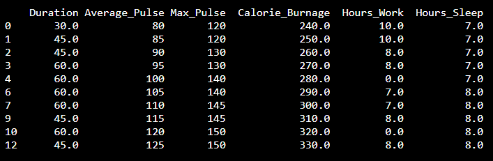
The result is a data set without NaN rows:
Data Categories
To analyze data, we also need to know the types of data we are dealing with.
Data can be split into two main categories:
- Quantitative Data - Can be expressed as a number or can be quantified. Can be divided into two sub-categories: Discrete data: Numbers are counted as "whole", e.g. number of students in a class, number of goals in a soccer game Continuous data: Numbers can be of infinite precision. e.g. weight of a person, shoe size, temperature
- Qualitative Data - Cannot be expressed as a number and cannot be quantified. Can be divided into two sub-categories: Nominal data: Example: gender, hair color, ethnicity Ordinal data: Example: school grades (A, B, C), economic status (low, middle, high)
By knowing the type of your data, you will be able to know what technique to use when analyzing them.
Data Types
We can use the info() function to list the data types within our data set:
Example
print(health_data.info())
Result:
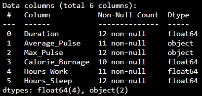
We see that this data set has two different types of data:
- Float64
- Object
We cannot use objects to calculate and perform analysis here. We must convert the type object to float64 (float64 is a number with a decimal in Python).
We can use the astype() function to convert the data into float64.
The following example converts "Average_Pulse" and "Max_Pulse" into data type float64 (the other variables are already of data type float64):
Example
  health_data["Average_Pulse"]
  = health_data['Average_Pulse'].astype(float)
health_data["Max_Pulse"] =
  health_data["Max_Pulse"].astype(float)

print
  (health_data.info())
Result:
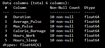
Now, the data set has only float64 data types.
Analyze the Data
When we have cleaned the data set, we can start analyzing the data.
We can use the describe() function in Python to summarize data:
Example
print(health_data.describe())
Result:
| Duration | Average_Pulse | Max_Pulse | Calorie_Burnage | Hours_Work | Hours_Sleep | |
|---|---|---|---|---|---|---|
| Count | 10.0 | 10.0 | 10.0 | 10.0 | 10.0 | 10.0 |
| Mean | 51.0 | 102.5 | 137.0 | 285.0 | 6.6 | 7.5 |
| Std | 10.49 | 15.4 | 11.35 | 30.28 | 3.63 | 0.53 |
| Min | 30.0 | 80.0 | 120.0 | 240.0 | 0.0 | 7.0 |
| 25% | 45.0 | 91.25 | 130.0 | 262.5 | 7.0 | 7.0 |
| 50% | 52.5 | 102.5 | 140.0 | 285.0 | 8.0 | 7.5 |
| 75% | 60.0 | 113.75 | 145.0 | 307.5 | 8.0 | 8.0 |
| Max | 60.0 | 125.0 | 150.0 | 330.0 | 10.0 | 8.0 |
- Count - Counts the number of observations
- Mean - The average value
- Std - Standard deviation (explained in the statistics chapter)
- Min - The lowest value
- 25%, 50% and 75% are percentiles (explained in the statistics chapter)
- Max - The highest value
