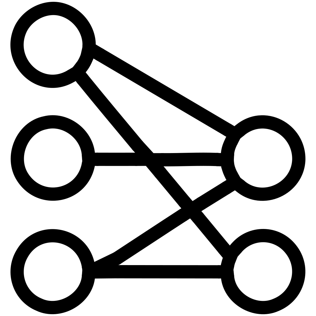
A sparse autoencoder takes a different approach to forcing a meaningful representation: instead of shrinking the latent dimension, allow it to be large (even larger than the input), but add a penalty that forces most of its individual units to stay inactive for any given input.
The Sparsity Penalty
\(\hat\rho_j\) is the average activation of latent unit \(j\) across a batch of training examples; \(\rho\) is a small target sparsity value (e.g. 0.05, meaning "on average, this unit should be active only 5% of the time"). The KL divergence term (see KL Divergence) penalizes any unit whose actual average activation drifts far from this small target — pushing most units toward mostly-inactive, with only a few "specializing" as active for any given input.
A Simpler Alternative: L1 Penalty on Activations
A more direct approach: add an L1 penalty (see L1 Regularization) directly on the latent activations themselves, which — recalling L1's tendency to push values to exactly zero — encourages most latent units to be exactly 0 for any given input, achieving a similar sparsity effect more simply.
Why Sparsity, Not Just Compression, Can Be Useful
A small bottleneck (plain autoencoder) forces compression, but the resulting features can be densely entangled — every unit contributes a little to every reconstruction. A large but sparse latent space instead encourages each individual unit to specialize, becoming meaningfully active only for specific, distinguishable patterns in the input — producing representations that can be more interpretable and more useful for certain downstream tasks, since each active unit tends to correspond to a more specific, identifiable feature.
Code
import torch
import torch.nn as nn

class SparseAutoencoder(nn.Module):
    def __init__(self, input_dim, latent_dim):
        super().__init__()
        self.encoder = nn.Sequential(nn.Linear(input_dim, latent_dim), nn.ReLU())   # latent_dim can be LARGE
        self.decoder = nn.Sequential(nn.Linear(latent_dim, input_dim), nn.Sigmoid())

    def forward(self, x):
        z = self.encoder(x)
        return self.decoder(z), z

model = SparseAutoencoder(input_dim=784, latent_dim=1000)   # latent dim LARGER than input
mse_loss = nn.MSELoss()

x = torch.rand(32, 784)
x_hat, z = model(x)
reconstruction_loss = mse_loss(x_hat, x)
sparsity_penalty = z.abs().mean()   # simple L1-style sparsity penalty on activations
total_loss = reconstruction_loss + 0.001 * sparsity_penalty
Common Mistakes
- Assuming a large latent dimension alone (without an explicit sparsity penalty) produces useful, disentangled features — without the penalty, a large latent space just makes the identity-function shortcut even easier to learn, exactly the failure mode a bottleneck was originally meant to prevent.
- Setting the sparsity coefficient \(\lambda\) too high — this can overly suppress activations, hurting reconstruction quality and effectively defeating the autoencoder's core purpose.
Interview Relevance
Q: "How does a sparse autoencoder force meaningful representation learning without shrinking the latent dimension?" Instead of relying on a small bottleneck to force compression, it allows a large (even oversized) latent space but adds an explicit penalty encouraging most latent units to stay inactive for any given input — via an L1 penalty on activations, or a KL-divergence penalty comparing each unit's average activation to a small target sparsity. This forces individual units to specialize rather than densely, redundantly contributing to every reconstruction.
Practice Question
Why might a sparse autoencoder's learned features be more interpretable than a plain, densely-compressed autoencoder's features?
