Hierarchical Clustering

Hierarchical Clustering

Hierarchical clustering is an unsupervised learning method for clustering data points. The algorithm builds clusters by measuring the dissimilarities between data. Unsupervised learning means that a model does not have to be trained, and we do not need a "target" variable. This method can be used on any data to visualize and interpret the relationship between individual data points.

Here we will use hierarchical clustering to group data points and visualize the clusters using both a dendrogram and scatter plot.

How does it work?

We will use Agglomerative Clustering, a type of hierarchical clustering that follows a bottom up approach. We begin by treating each data point as its own cluster. Then, we join clusters together that have the shortest distance between them to create larger clusters. This step is repeated until one large cluster is formed containing all of the data points.

Hierarchical clustering requires us to decide on both a distance and linkage method. We will use euclidean distance and the Ward linkage method, which attempts to minimize the variance between clusters.

Example

  import numpy as np
import matplotlib.pyplot as plt

x = [4, 5, 10, 4,
  3, 11, 14 , 6, 10, 12]
y = [21, 19, 24, 17, 16, 25, 24, 22, 21, 21]

  plt.scatter(x, y)
plt.show()

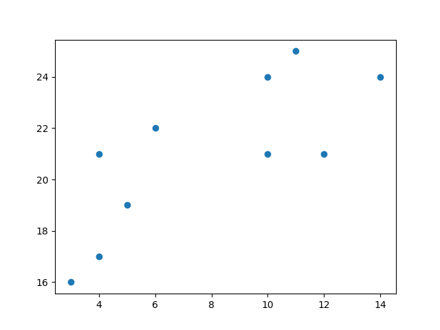
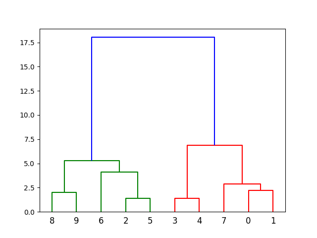
Now we compute the ward linkage using euclidean distance, and visualize it using a dendrogram:

Example

  import numpy as np
import matplotlib.pyplot as plt
from
  scipy.cluster.hierarchy import dendrogram, linkage

x = [4, 5, 10, 4, 3,
  11, 14 , 6, 10, 12]
y = [21, 19, 24, 17, 16, 25, 24, 22, 21, 21]

  data = list(zip(x, y))

linkage_data = linkage(data, method='ward',
  metric='euclidean')
dendrogram(linkage_data)

plt.show()

Example

  import numpy as np
import matplotlib.pyplot as plt
from sklearn.cluster
  import AgglomerativeClustering

x = [4, 5, 10, 4, 3, 11, 14 , 6, 10, 12]
  y = [21, 19, 24, 17, 16, 25, 24, 22, 21, 21]

data = list(zip(x, y))

hierarchical_cluster = AgglomerativeClustering(n_clusters=2,
  linkage='ward')
labels = hierarchical_cluster.fit_predict(data)

  plt.scatter(x, y, c=labels)
plt.show()

Example Explained

Import the modules you need.

<p><code class="pythonHigh">import numpy as np<br/>
import matplotlib.pyplot as plt<br/>
from scipy.cluster.hierarchy import dendrogram, linkage<br/>
from sklearn.cluster import AgglomerativeClustering</code></p>

You can learn about the Matplotlib module in our "Matplotlib Tutorial.

You can learn about the SciPy module in our SciPy Tutorial.

NumPy is a library for working with arrays and matricies in Python, you can learn about the NumPy module in our NumPy Tutorial.

scikit-learn is a popular library for machine learning.

Create arrays that resemble two variables in a dataset. Note that while we only use two variables here, this method will work with any number of variables:

<p><code class="pythonHigh">x = [4, 5, 10, 4, 3, 11, 14 , 6, 10, 12]<br/>
y = [21, 19, 24, 17, 16, 25, 24, 22, 21, 21]
</code></p>

Turn the data into a set of points:

<p><code class="pythonHigh">data = list(zip(x, y))<br/>
print(data)
</code></p>

Result:

<p><code class="pythonHigh">[(4, 21), (5, 19), (10, 24), (4, 17), (3, 16), (11, 25), (14, 24), (6, 22), (10, 21), (12, 21)]
</code></p>

Compute the linkage between all of the different points. Here we use a simple euclidean distance measure and Ward's linkage, which seeks to minimize the variance between clusters.

<p><code class="pythonHigh">linkage_data = linkage(data, method='ward', metric='euclidean')
</code></p>

Finally, plot the results in a dendrogram. This plot will show us the hierarchy of clusters from the bottom (individual points) to the top (a single cluster consisting of all data points).

plt.show() lets us visualize the dendrogram instead of just the raw linkage data.

<p><code class="pythonHigh">dendrogram(linkage_data)<br/>
plt.show()
</code></p>

Result:

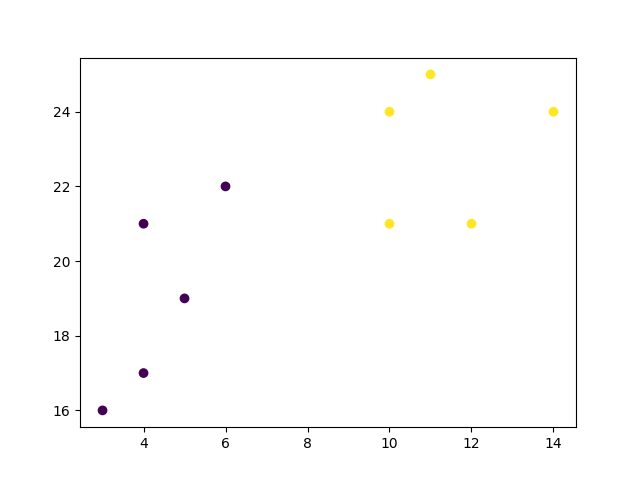
The scikit-learn library allows us to use hierarchichal clustering in a different manner. First, we initialize the AgglomerativeClustering class with 2 clusters and the Ward linkage.

<p><code class="pythonHigh">hierarchical_cluster = AgglomerativeClustering(n_clusters=2, linkage='ward')
</code></p>

The .fit_predict method can be called on our data to compute the clusters using the defined parameters across our chosen number of clusters.

<p><code class="pythonHigh">labels = hierarchical_cluster.fit_predict(data)
print(labels)
</code></p>

Result:

<p><code class="pythonHigh">[0 0 1 0 0 1 1 0 1 1]
</code></p>

Finally, if we plot the same data and color the points using the labels assigned to each index by the hierarchical clustering method, we can see the cluster each point was assigned to:

<p><code class="pythonHigh">plt.scatter(x, y, c=labels)<br/>
plt.show()
</code></p>

Result: